Distributions

The distribution of a variable is a description of the relative numbers of times each possible outcome will occur in a number of trials.
The function describing the probability that a given value will occur is called the probability density function (abbreviated PDF), and the function describing the cumulative probability that a given value or any value smaller than it will occur is called the distribution function (or cumulative distribution function, abbreviated CDF).
Note: The probability that a certain "discrete" random variable will take is given by the probability mass function (abbreviated PMF).

Discrete Distribution

A discrete distribution is a distribution of data in statistics that has discrete values. Discrete values are countable, finite, non-negative integers, such as 1, 10, 15.
The most common discrete distributions used by statisticians or analysts include the Bernoulli, Binomial and the Poisson distributions. Others include the Multinomial, Negative Binomial, Geometric, and Hypergeometric distributions.

1. Bernoulli Distribution

A Bernoulli distribution has only two possible outcomes, namely $1$ (success) and $0$ (failure), and a single trial, for example, a coin toss. So the random variable $X$ which has a Bernoulli distribution can take value $1$ with the probability of success, $p$, and the value $0$ with the probability of failure, $q$ or $1-p$. The probabilities of success and failure need not be equally likely. The Bernoulli distribution is a special case of the binomial distribution where a single trial is conducted ($n=1$).
Its probability mass function, PMF is given by: $$\text{pmf}(x, p) = \left\{\begin{matrix} p & \text{if} \ x = 1\\ 1 - p & \text{if} \ x = 0 \end{matrix}\right.$$

Its cumulative distribution function, CDF is given by: $$ \text{cdf}(x, p) = \left\{\begin{matrix} 0 & \text{if} \ x < 0 \\ 1 - p & \text{if} \ 0 \leq x < 1 \\ p & \text{if} \ x \geq 1 \end{matrix}\right.$$

import numpy as np
import matplotlib.pyplot as plt
from scipy.stats import bernoulli

p = 0.3

x = [0, 1]
y = bernoulli.pmf(x, p)

plt.scatter(x, y)
plt.xlabel('x')
plt.ylabel('PMF (Probability)')
plt.show()

x = [-1, 0, 0.5, 1, 1.5]
y = bernoulli.cdf(x, p)
plt.scatter(x, y)
plt.xlabel('x')
plt.ylabel('CDF (Cumulative Probability)')
plt.show()

2. Binomial Distribution

It describes the outcome of binary scenarios, e.g. toss of a coin, it will either be head or tails.
The formula for binomial distribution is as follows,

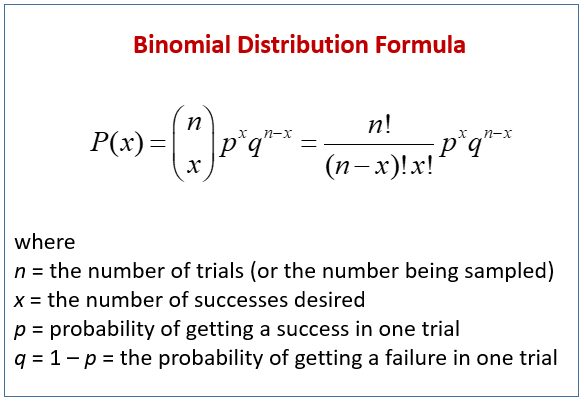
For a binomial distribution, the mean, variance and standard deviation for the given number of success are represented using the formulas

• Mean, $\mu = np$
• Variance, ${\sigma}^{2} = npq$
• Standard Deviation, $\sigma = \sqrt{npq}$

Properties of Binomial Distribution:

• There are two possible outcomes: true or false, success or failure, yes or no.
• There is ‘n’ number of independent trials or a fixed number of n times repeated trials.
• The probability of success or failure remains the same for each trial.
• Only the number of success is calculated out of n independent trials.
• Every trial is an independent trial, which means the outcome of one trial does not affect the outcome of another trial.

import numpy as np
import matplotlib.pyplot as plt
from collections import Counter
from scipy.stats import binom

n = 10
p = 0.5

random_variates = binom.rvs(n, p, size=10000)
freq = Counter(random_variates)

plt.bar(freq.keys(), freq.values())
plt.xlabel('x')
plt.ylabel('Frequency')
plt.show()

x = range(1, n + 1)
y = binom.pmf(x, n, p)

plt.bar(x, y)
plt.xlabel('x')
plt.ylabel('PMF (Probability)')
plt.show()

y = binom.cdf(x, n, p)

plt.bar(x, y)
plt.xlabel('x')
plt.ylabel('CDF (Cumulative Probablity)')
plt.show()

Continuous Distribution

A continuous distribution describes the probabilities of the possible values of a continuous random variable. A continuous random variable is a random variable with a set of possible values (known as the range) that is infinite and uncountable.
Probabilities of continuous random variables (X) are defined as the area under the curve of its PDF. Thus, only ranges of values can have a non-zero probability. The probability that a continuous random variable equals some value is always zero.

This is a comparison between disrete distribution and continous normal distribution

In the case of a continuous distribution, the values are present in an infinite range. Thus, in a continuous distribution, the numbers are infinite.

1. Normal Distribution

Normal distribution, also known as the Gaussian distribution, is a probability distribution that is symmetric about the mean, showing that data near the mean are more frequent in occurrence than data far from the mean. In graph form, normal distribution will appear as a bell curve.
The formula for normal distribution is as follows,

Where,

• $x$ is the variable
• $\mu$ is the mean
• $\sigma$ is the standard deviation

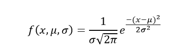
Some of the important properties of the normal distribution are listed below:

• In a normal distribution, the mean, median and mode are equal.(i.e., Mean = Median= Mode).
• The total area under the curve should be equal to 1.
• The normally distributed curve should be symmetric at the centre.
• There should be exactly half of the values are to the right of the centre and exactly half of the values are to the left of the centre.
• The normal distribution should be defined by the mean and standard deviation.
• The normal distribution curve must have only one peak. (i.e., Unimodal)
• The curve approaches the x-axis, but it never touches, and it extends farther away from the mean.

The normal distributions are closely associated with many things such as:

• Marks scored by students.
• Heights of different people.
• Blood pressure and so on.

import numpy as np
import matplotlib.pyplot as plt
from scipy.stats import norm

mu = 50
sigma = 10

x = np.arange(1, 100, 1)
y = norm.pdf(x, loc=mu, scale=sigma)

plt.plot(x, y)
plt.xlabel('x')
plt.ylabel('PDF (Probability)')
plt.show()

y = norm.cdf(x, loc=mu, scale=sigma)

plt.plot(x, y)
plt.xlabel('x')
plt.ylabel('CDF (Cumulative Probability)')
plt.show()

random_variates = norm.rvs(loc=mu, scale=sigma, size=100)

plt.hist(random_variates, bins=range(0, 110, 10))
plt.show()

KDE & ECDF !

Kernel Density Estimation and Empirical (Cumulative) Distribution Function

KDE: Kernel density estimation is a way to estimate the probability density function (PDF) of a random variable in a non-parametric (do not rely on particular methods of any particular parametric family of probability distributions) way. Link

ECDF: The empirical distribution function is an estimate of the cumulative distribution function that generated the points in the sample.

sample = [
    45.72890767, 57.54074   , 57.74424154, 49.01023188, 65.82064244,
    74.64647005, 71.43935562, 56.56965998, 62.74854826, 62.74497962,
    55.32891303, 58.50888097, 56.4870966 , 36.30498791, 55.35951074,
    58.78489198, 58.05612933, 65.92703362, 58.14252147, 71.53713032,
    60.10056839, 65.52252553, 71.2515607 , 65.36640035, 63.85298975,
    58.62577178, 57.1900372 , 60.69841172, 57.46680469, 54.54782006,
    64.63465735, 51.92483114, 64.48192516, 59.02304139, 54.54468221,
    60.10394962, 74.3345832 , 51.74661325, 60.9057343 , 65.26049855,
    48.20977518, 51.55121313, 59.16774611, 85.5000865 , 58.57799841,
    56.54318968, 41.00254418, 61.55473646, 66.64809434, 47.75680707, 
    15.43483718, 16.13186908, 15.57226928, 12.41345967, 26.58716259,
    23.88670474, 23.14018873, 18.279609  , 22.55012777, 25.68339096,
    11.24359196, 17.57701799, 17.34347412, 30.36664984, 22.16632605,
    14.83508626, 21.75400292, 26.15033607, 18.20081078, 31.91644308,
    22.47250516, 20.02148907, 15.55271268, 18.27857685, 20.9660308 ,
    25.83615163, 22.08327585, 21.46572823, 23.90567488, 17.3321409 ,
    20.32825321, 27.04990061, 18.66636605, 28.76709141, 21.69811349,
    25.29080758, 13.22075277, 12.82817099, 22.44913153, 14.2253315 ,
    14.90517892, 16.3680904 , 16.13615834, 21.52562982, 22.22446452,
    18.7617733 , 22.88582609,  9.87183471, 24.12320574, 24.06825282]

plt.hist(sample, bins=range(0, 100, 5))
plt.show()

from scipy.stats import gaussian_kde

kde = gaussian_kde(sample)

x = np.arange(0, 100, 0.1)
y = kde.pdf(x)

print(sum(y))

plt.plot(x, y)
plt.xlabel('x')
plt.ylabel('PDF (Probability)')
plt.show()

9.907966533793271

from scipy.stats import ecdf

res = ecdf(sample)

print(f"\n Quantiles: {res.cdf.quantiles}")
print(f"\n Probabilities: {res.cdf.probabilities}")

 Quantiles: [ 9.87183471 11.24359196 12.41345967 12.82817099 13.22075277 14.2253315
 14.83508626 14.90517892 15.43483718 15.55271268 15.57226928 16.13186908
 16.13615834 16.3680904  17.3321409  17.34347412 17.57701799 18.20081078
 18.27857685 18.279609   18.66636605 18.7617733  20.02148907 20.32825321
 20.9660308  21.46572823 21.52562982 21.69811349 21.75400292 22.08327585
 22.16632605 22.22446452 22.44913153 22.47250516 22.55012777 22.88582609
 23.14018873 23.88670474 23.90567488 24.06825282 24.12320574 25.29080758
 25.68339096 25.83615163 26.15033607 26.58716259 27.04990061 28.76709141
 30.36664984 31.91644308 36.30498791 41.00254418 45.72890767 47.75680707
 48.20977518 49.01023188 51.55121313 51.74661325 51.92483114 54.54468221
 54.54782006 55.32891303 55.35951074 56.4870966  56.54318968 56.56965998
 57.1900372  57.46680469 57.54074    57.74424154 58.05612933 58.14252147
 58.50888097 58.57799841 58.62577178 58.78489198 59.02304139 59.16774611
 60.10056839 60.10394962 60.69841172 60.9057343  61.55473646 62.74497962
 62.74854826 63.85298975 64.48192516 64.63465735 65.26049855 65.36640035
 65.52252553 65.82064244 65.92703362 66.64809434 71.2515607  71.43935562
 71.53713032 74.3345832  74.64647005 85.5000865 ]

 Probabilities: [0.01 0.02 0.03 0.04 0.05 0.06 0.07 0.08 0.09 0.1  0.11 0.12 0.13 0.14
 0.15 0.16 0.17 0.18 0.19 0.2  0.21 0.22 0.23 0.24 0.25 0.26 0.27 0.28
 0.29 0.3  0.31 0.32 0.33 0.34 0.35 0.36 0.37 0.38 0.39 0.4  0.41 0.42
 0.43 0.44 0.45 0.46 0.47 0.48 0.49 0.5  0.51 0.52 0.53 0.54 0.55 0.56
 0.57 0.58 0.59 0.6  0.61 0.62 0.63 0.64 0.65 0.66 0.67 0.68 0.69 0.7
 0.71 0.72 0.73 0.74 0.75 0.76 0.77 0.78 0.79 0.8  0.81 0.82 0.83 0.84
 0.85 0.86 0.87 0.88 0.89 0.9  0.91 0.92 0.93 0.94 0.95 0.96 0.97 0.98
 0.99 1.  ]

plt.plot(res.cdf.quantiles, res.cdf.probabilities)
plt.xlabel('x')
plt.ylabel('ECDF')
plt.show()